Cyclical Statistical Forecasts and Anomalies – Part 6

That’s right, because unfortunately not all data is created equally—different profiles, periodicity and underlying characteristics mean that anomaly detection can be a varied field for us here at Splunk. Even recently you may have seen some methods for generating baselines, statistics and likelihoods on big data along side a decision tree for selecting the right way to detect anomalies.

Despite this variety of approaches, we often have situations where “some of the alerts generated by the existing configuration are false positives, leading to alert fatigue, false interpretation, and improper resource utilization” according to Manish Mittal, a Senior Data Scientist with GovCIO.

It is Manish’s fine work that has inspired this blog post, where he has been looking to detect anomalies in counts of events that occur independently of each other. Now there is a lot to unpack in terms of what that means, but we are talking about situations like:

• • Users logging on to a system.
  • Error rates from a web application.
  • Number of distinct network connections over time.
  • Users making purchases on a website.
  • Event counts of data coming into Splunk.

These are very different to continuous variables, such as CPU utilization or session durations, which would be entirely unsuitable for the technique we’re about to take you through.

Although we’d often suggest using the Machine Learning Toolkit for capturing baselines using the fit command, here we’re going to take a slightly different approach using core SPL and lookups.

Like almost all machine learning methods the first step for us is to train a model or capture some descriptive statistics from historic data. The statistics that we are interested in are:

• The average number of events, as this tells us what the baseline is for us to track to.
• The number of records used to generate the average, as we can use this to filter out ‘noise’ – in this case averages that have been calculated on a sample size that is too small to be meaningful.

In this example we will be using all 31 days worth of data from the BOTSv2 data to collect some information about the average number of events generated by sourcetype for a given hour of day and day of the week. The search can be seen below, where we are counting the number of events over each 10 minute interval for each sourcetype. We then create a key for each sourcetype, hour and day combination, and remove the upper 95th percentile of the data to try and remove some outliers from our training dataset. Once we’ve done some basic outlier removal we are collecting our baseline statistics — the average value and the number of records used to calculate the average — into a lookup.

In our example there are just over 12k keys in our lookup, which works just fine as a csv lookup. In Manish’s real world example he had over 100k keys, which is much better stored in the KV store to avoid performance issues associated with huge knowledge objects – like large csv lookups. If you want to know more about the benefits of using the KV Store for situations like these Josh Cowling takes you through some of the ins and outs in his blog here.

Now that we have our lookup we’re going to use it to enrich new data with the average and cardinality that we have seen from the historic data. Applying a filter based on the cardinality we are going to ignore data that has averages based on less than 10 historic records. Note that this is done behind the scenes with the DensityFunction algorithm in MLTK, where we recommend having a cardinality of 50 or more and actually don’t detect outliers in data that has cardinality less than 15. Removing these low cardinality data points means that we are now looking only at records that we have reasonable confidence in as we have seen plenty of historic data from them in the past.

With our current data we are going to use the count of events and the average count of events to calculate a probability of the current count occurring. To do this we are modeling the data as having a Poisson Distribution, and have some SPL to determine the probability based on this distribution. To do this we need to calculate the factorial of the current event count (using Stirling’s approximation) and the exponential of the negative mean, and while this may seem like a lot of complicated mathematics don’t worry – we’ve provided the SPL below. From these two values we can now determine the probability, and have chosen to flag outliers as event counts that have a probability of less than 0.3%.

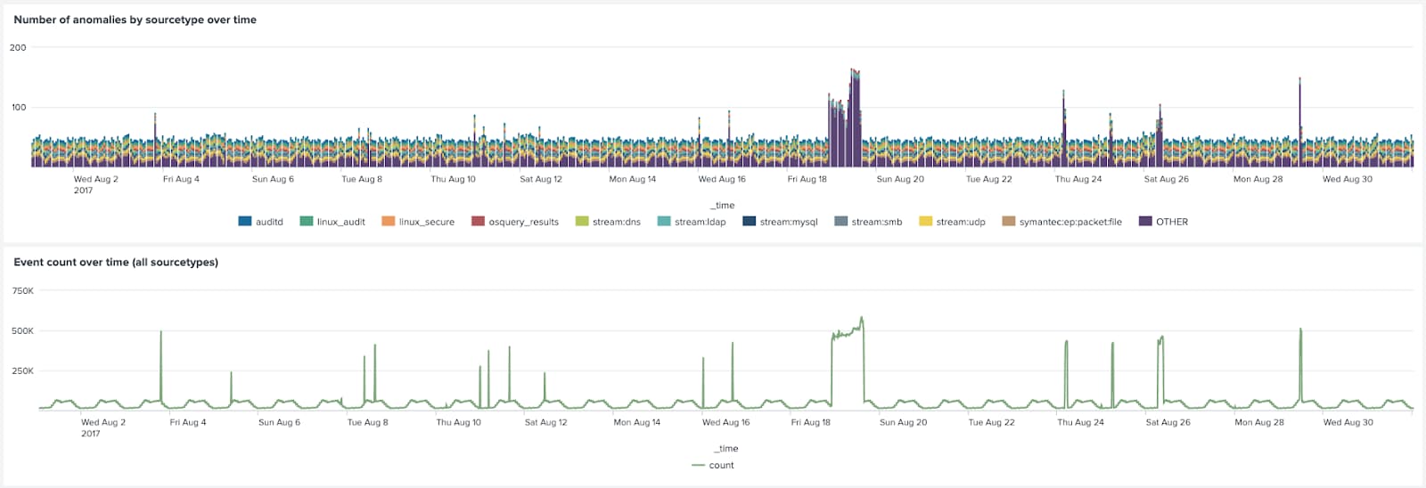
As can be seen in the chart below the number of outliers by sourcetype is a very close match to the overall event count over time in the BOTSv2 data.

This part is really simple, just go and try out the SPL above on your own indexed data! You may need to select an index that has data actively coming into it to base your searches on, and make sure to select a long time period (30 days or more) for your initial search to generate the lookup.

To learn more about the technique discussed in this blog please come along to our talk at .conf22, where Manish, Pinar and I will be talking through how you can use ML in Splunk to discover new insights like this. While you’re at it, why not come along to .conf to find out about how other customers are using ML to get more out of their data!

If you are interested in alternative methods of detecting outliers in data streams coming into Splunk check out our webinar on preventing data downtime with machine learning, or the Machine Learning Toolkit (MLTK) tutorial of the very same topic.

Alternatively if anomaly detection is your thing please read the previous five entries in this series, or watch back our tech talk on anomaly detection with Splunk machine learning.

Happy Splunking!